Regression Exercise #2

Simulate some data

If you’re feeling up to it, follow the guidelines below to generate some data. If not, take a look at the solution and skip to the next section. Let’s generate some sample data, which we will use to estimate parameters of a linear model using ordinary least squares (OLS). Create a function called generate_data() that takes in a single argument, n, which represents the sample size of our simulated data. In this function:

1. Draw the variables for age, income, and bwt (birthweight) according to the expressions given below.
2. Return age, income, and bwt in a data frame object.

\[\begin{align*} \texttt{age} &= \text{Uniform}(min = 25, max = 60) \\ \texttt{income} &= (\texttt{age} \times 500) \\ &\ \ \ \ \ \ \ + \text{Beta}(shape1 = 2, shape2 = 3.46, ncp = 0) \times 100000 \\ &\ \ \ \ \ \ \ - 15000 \\ \texttt{bwt} &= 2450 + (\texttt{income/1000}) \times 14 \\ &\ \ \ \ \ \ \ - (\texttt{age} \times 2) + \text{Normal}(mean = -100, sd = 100) \end{align*}\]

The runif() function in R draws realizations of the Uniform distribution, the rbeta() function draws realizations of the Beta distribution, and the rnorm() function draws realizations of the Normal distribution.

Set the random seed to 1, i.e. (set.seed(1)). Using the generate_data() function you just created, draw n=1000 observations and assign the data to a data.frame object called dat.

Choose a statistical model

Take a look at the variables found in dat, using the summary() function. Examine the first 6 rows of the data using the head() function. Create a scatter plot with dat$age on the x-axis and dat$bwt on the y-axis, using the plot() function.

In this case, does a linear relationship between age and bwt seem reasonable?

OLS Part 1: Implement using lm()

The lm() function in R estimates parameters from linear models using ordinary least squares. There are two main structural arguments for this function, formula, and data.

• The data argument is straightforward, and should be a data.frame object that holds your variables.
• The formula argument should be formatted as: outcomeVar ~ explanatoryVar, and tells R which variable is the outcome and which are covariates (separated by the “~” symbol).

For example, we call the function and assign it to the object, fit.object below. When we call the summary() function on our fit.object, R returns useful information about the procedure and presents some key results.

fit.object <- lm(outcome ~ exposure + covariate1 + covariate2 ..., data = mydata)
summary(fit.object)

Using the lm() function, estimate the parameters from a regression model with OLS with birthweight (bwt) as the outcome and age as the single covariate. Assume a linear relationship between birthweight and age. Assign the results from this procedure a new object, ols.fit, then call summary() on this new object.

What do you conclude about the relationship between age and birthweight? How do you interpret the coefficient for age?

OLS Part 2: Functional form

In the previous section, we assumed a linear relationship between age and birthweight. What if we assumed a quadratic relationship instead? Repeat the regression analysis from above, this time also including a second covariate for squared age. There are multiple options for creating this variable:

• Generate a variable age_squared in our dat dataset by multiplying the age variable by itself, then include this term in our formula expression.

dat$age_squared <- dat$age * dat$age

• Create this variable when we specify our formula in lm(), using the I() function. The I() function (see ?I for more info) tells R to evaluate whatever is inside its parentheses before including it in the formula. Without it, R ignores the fact that we would like a term for squared age.

ols.fit_squared <- lm(bwt ~ age + I(age^2), data = dat)

Repeat the previous analysis from Part 1, this time with a second covariate for squared age, and save the results to ols.fit_squared. Call summary() on this object to look at the results, what do you conclude?

OLS Part 3: Confounding

Now let’s say we’re interested in the effect, not just the association, between age and birthweight. AND let’s assume that the only source of potential confounding for the age-birthweight relationship is income (in reality this is unlikely). Repeat the regression analysis from Part 1, but this time include the covariate income in your regression equation. Save your results to a new object, ols.fit_income, and look at the results.

How does the coefficient for age differ between Part 1 and Part 3? Why do you think this is the case? (hint: look at the simulation set up before Part 1).

Visualizing Models

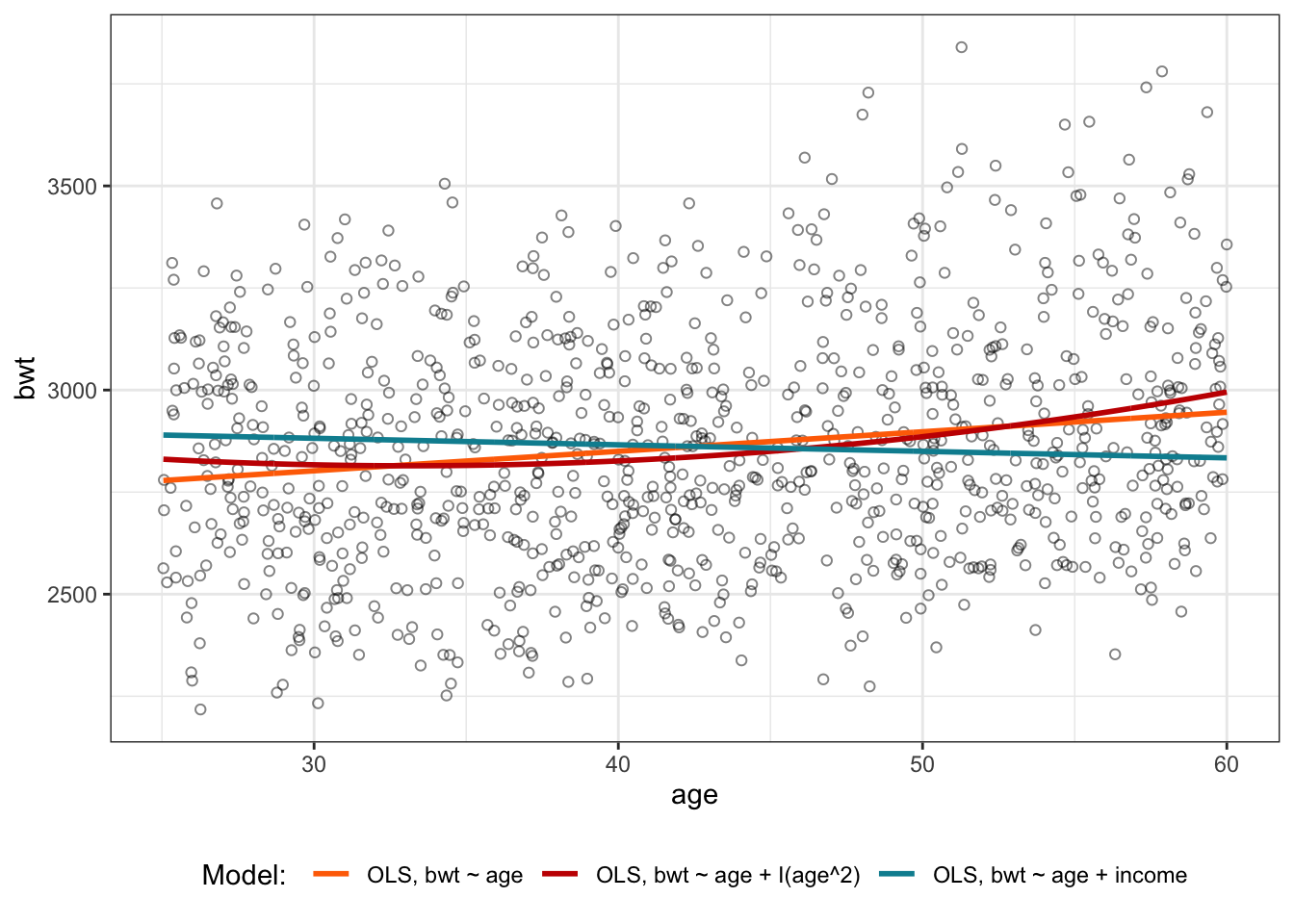
A useful step in model building is to plot the results of our estimation alongside the observed data, in order to make sure our results are sensible. The code below plots the predicted lines from each of the 3 models we ran, against a scatter plot of age vs. birthweight. The fitted values of birthweight for the last model, with income as a covariate, is predicted at the mean income for the dataset.

library(ggplot2)
library(dplyr)
library(ggsci)
library(reshape2)
library(tidyr)
library(data.table)

# load data
set.seed(1)
dat <- generate_data(n = 1000)

# fits
ols.fit <- lm(bwt ~ age, data = dat)
ols.fit_squared <- lm(bwt ~ age + I(age^2), data = dat)
ols.fit_income <- lm(bwt ~ age + income, data = dat)

# predictions according to each model
pred.dat <- dat
pred.dat <- 
  pred.dat %>% 
  mutate(income = mean(income))

pred.dat$yhat_ols1 <- predict(ols.fit, newdata = pred.dat, se.fit = FALSE, "response")
pred.dat$yhat_ols2 <- predict(ols.fit_squared, newdata = pred.dat, se.fit = FALSE, "response")
pred.dat$yhat_ols3 <- predict(ols.fit_income, newdata = pred.dat, se.fit = FALSE, "response")

# convert to long dataset for plotting
id.vars <- c("age", "income", "bwt")
measure.vars <- 
  list(
    prediction = c('yhat_ols1', 'yhat_ols2', 'yhat_ols3')
  )
pred.dat.long <- 
  reshape2::melt(
    setDT(pred.dat),
    id.vars = id.vars,
    measure.vars = measure.vars,
    variable.name = "Model: ")
pred.dat.long$`Model: ` <- factor(
  pred.dat.long$`Model: `,
  labels = c("OLS, bwt ~ age", 
             "OLS, bwt ~ age + I(age^2)",
             "OLS, bwt ~ age + income")
)

# plot using ggplot2
ggplot(pred.dat.long[1:3000,], 
       aes(x = age, y = bwt, color = `Model: `, group = `Model: `)) + 
  geom_point(color = "black", shape = 21, alpha = 0.2) + 
  geom_line(aes(x = age, y = value), size = 1) + 
  theme_bw() + 
  scale_color_futurama() + 
  theme(legend.position = "bottom")